Examples

In this short tutorial is shown the results of the ENIIGMA code applied to the YSO SVS 4-9, located in the SVS4 cluster in the Serpens molecular cloud.

The L-band spectrum data was taken from the VLT-ISAAC public database via this link. The near-IR photometric data is available in the 2MASS catalog.

Note

These examples aim to show the code’s functionalities and should not be taken as an accurate scientific result!

Polynomial continuum

In order to calculate the continuum SED an calculate the optical depth using the polynomial function, we can use the following command:

>>> from ENIIGMA.Continuum import Fit
>>> filename = '/Users/will_rocha_starplan/eniigma_doc/doc/Tutorial/svs49.txt'
>>> Fit.Continuum_poly(filename, 1.24, 4.0, order = 2., range_limits=[[1.24, 2.85], [3.8, 4.]])

The parameters indicate that the continuum is calculated in the range between 1.24 to 4.0 microns, using a second-order polynomial function constrained by the ranges between 1.24-2.85 and 3.8-4. microns.

The results are shown below:

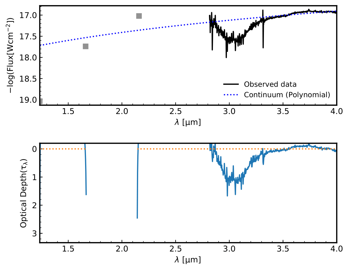
Figure 1: Continuum SED, SVS4-9 spectrum on the top panel, the optical depth on the bottom panel.

As you can note, the function fails to trace the continuum in the near-IR regime, althout it gives an acceptable continuum in the L-band interval. Below the same procedure is repeated using the blackbody function.

Blackbody continuum

The Python commands to call the BB continuum function is:

>>> from ENIIGMA.Continuum import Fit
>>> Fit.Continuum_BB(filename, 1.24, 4., range_limits=[[1.25, 2.5], [3.8, 4.]], guess = (1000, 1e-20))

As used in the polynomial continuum case, the intervals are the same. The difference is that one BB function is used. The initial guesses to fit the spectrum are the temperature of 1000 K and a scale factor of 1e-20. The results are shown below:

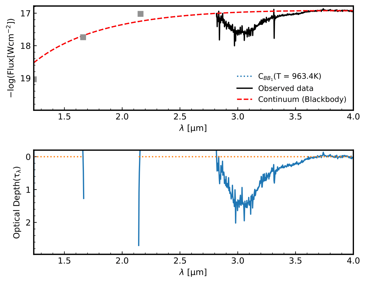
Figure 2: Continuum SED, SVS4-9 spectrum on the top panel, the optical depth on the bottom panel.

GA decomposition

The spectral decomposition using the genetic algorithm module reads the output from the polynomial continuum and BB function as well as an external file not calculated by the ENIIGMA code. As example, let us use the output spectrum from the ENIIGMA code.

>>> from ENIIGMA.GA import optimize
>>> filename = 'Optical_depth_svs49.od'
>>> list_sp = ['H2O_40K', 'H2O_NH3_CO2_CH4_10_1_1_1_72K_b', 'd_NH3_CH3OH_50_10K_I10m_Baselined', 'CO_NH3_10K', 'H2O_CH4_10_0.6_a_V3', 'CO_CH3OH_10K', 'HNCO_NH3']
>>> optimize.ENIIGMA(filename, 2.84, 4., list_sp, group_comb=3, skip=False, pathlib = None)

The optical depth used in this example is the file ‘Optical_depth_svs49.od’, and the initial guess for the laboratory data are listed in the list_sp variable. Once the files are set, the decomposition range is fixed for the interval between 2.84 and 4. microns, with a combination group of 3 experimental data in the final step of the code. The keyword ‘skip=False’ means that the entire procedure will be executed. ‘pathlib=None’ means that the ice library is read from the folder download with the code. It is stored in your Python directory. Alternatively you can download the ice library here.

In my laptop, 156 combinations were tested in a execution time of 75 seconds. The result is shown below:

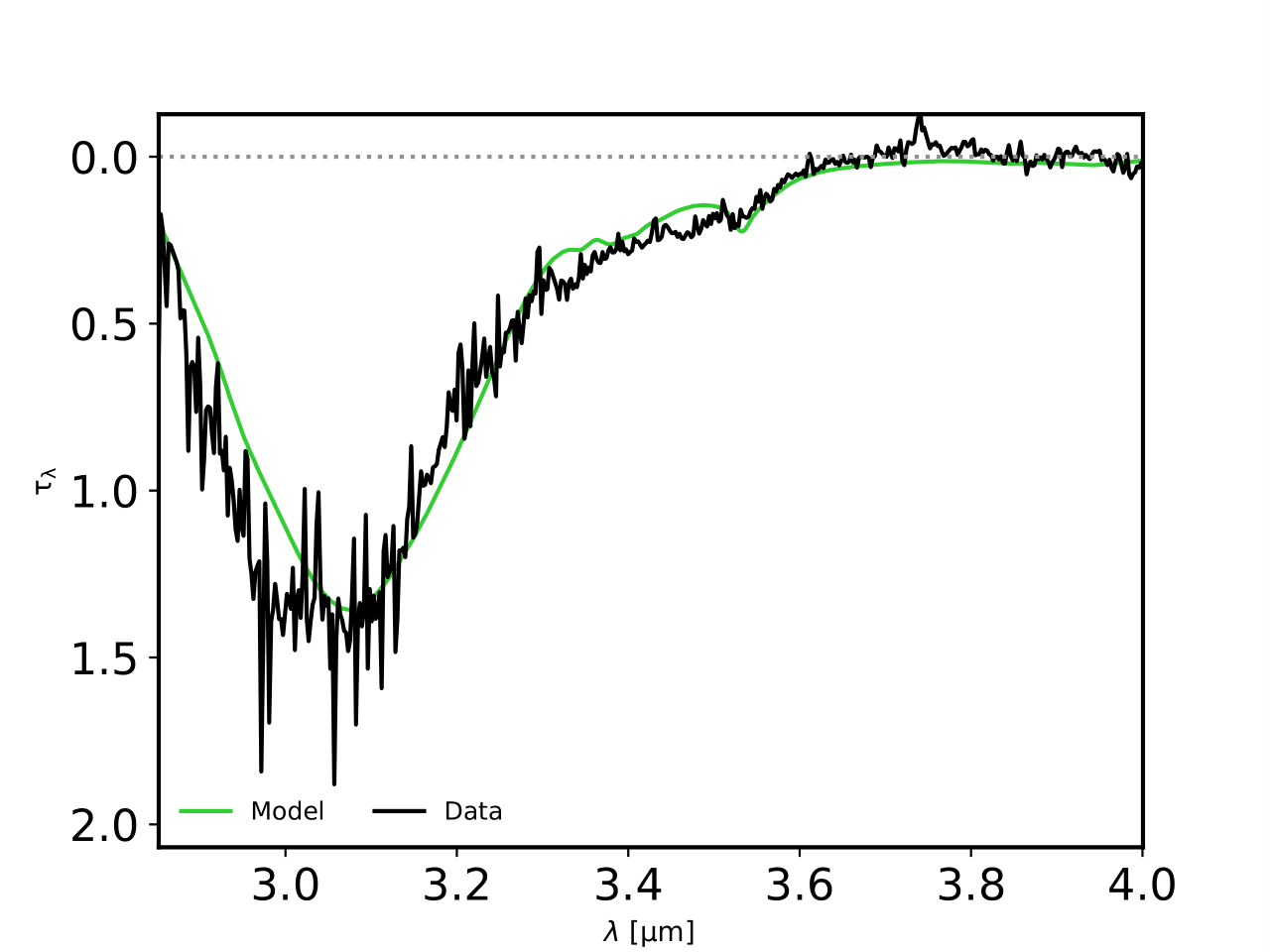
Figure 3: SVS 4-9 optical depth in black and the fitting model in green.

Checking out the GA fitness evolution

The evolution of the optimisation over the generations for the combinations can be checked in two different ways. First, the 5 best combinations can be checked via this command:

>>> from ENIIGMA.GA import check_ga
>>> check_ga.top_five_scaled(savepdf=True)

This will show the 5 best scaled fitness function in the same graph as seen below:

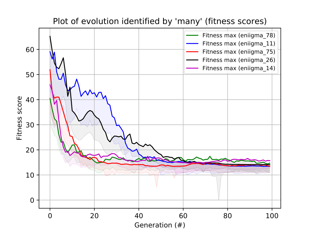
Figure 4: GA evolution check.

Other checking options are available via this command:

>>> from ENIIGMA.GA import check_ga
>>> check_ga.check(combination=78, option=-4)

The figure below shows the evolution of the combination that gave the best solution, namely - 78.

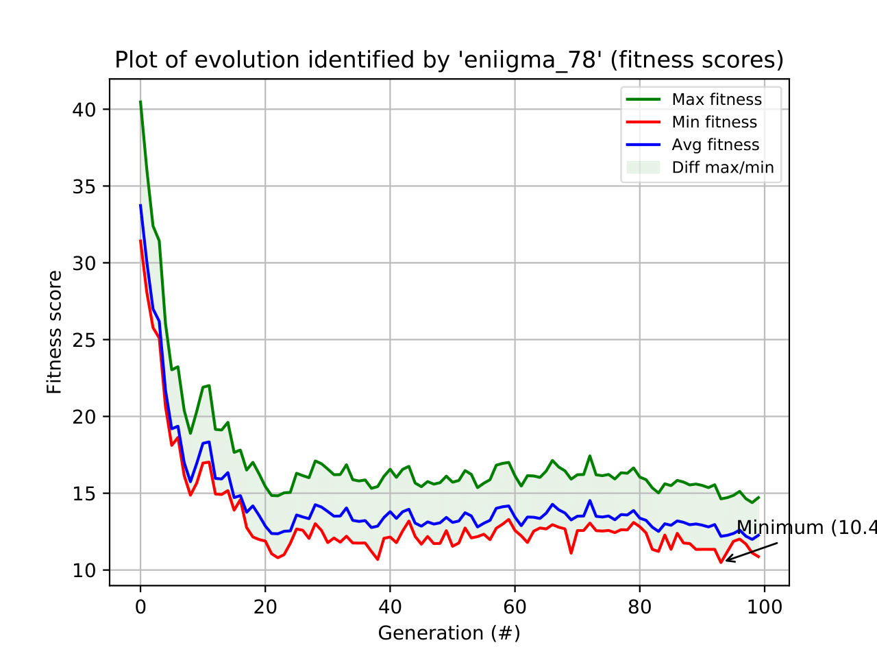
Figure 5: GA evolution check for the best combination.

The population evolution can also be check over the generations and fitness function as follows:

>>> from ENIIGMA.GA import check_ga
>>> check_ga.check(combination=78, option=-9)

The result is shown below:

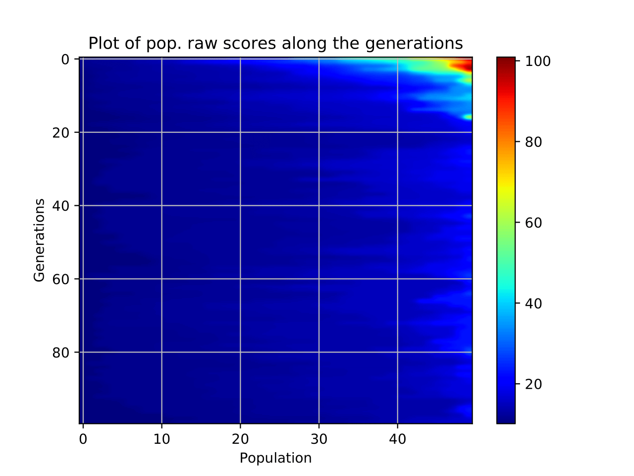
Figure 6: Population check for the best combination.

Evaluating the recurrence of the ice components

The recurrence of the ice laboratory inside the confidence intervals can be addressed via pie charts. For example:

>>> from ENIIGMA.Stats import Pie_chart_plots
>>> Pie_chart_plots.pie(sig_level=9.)

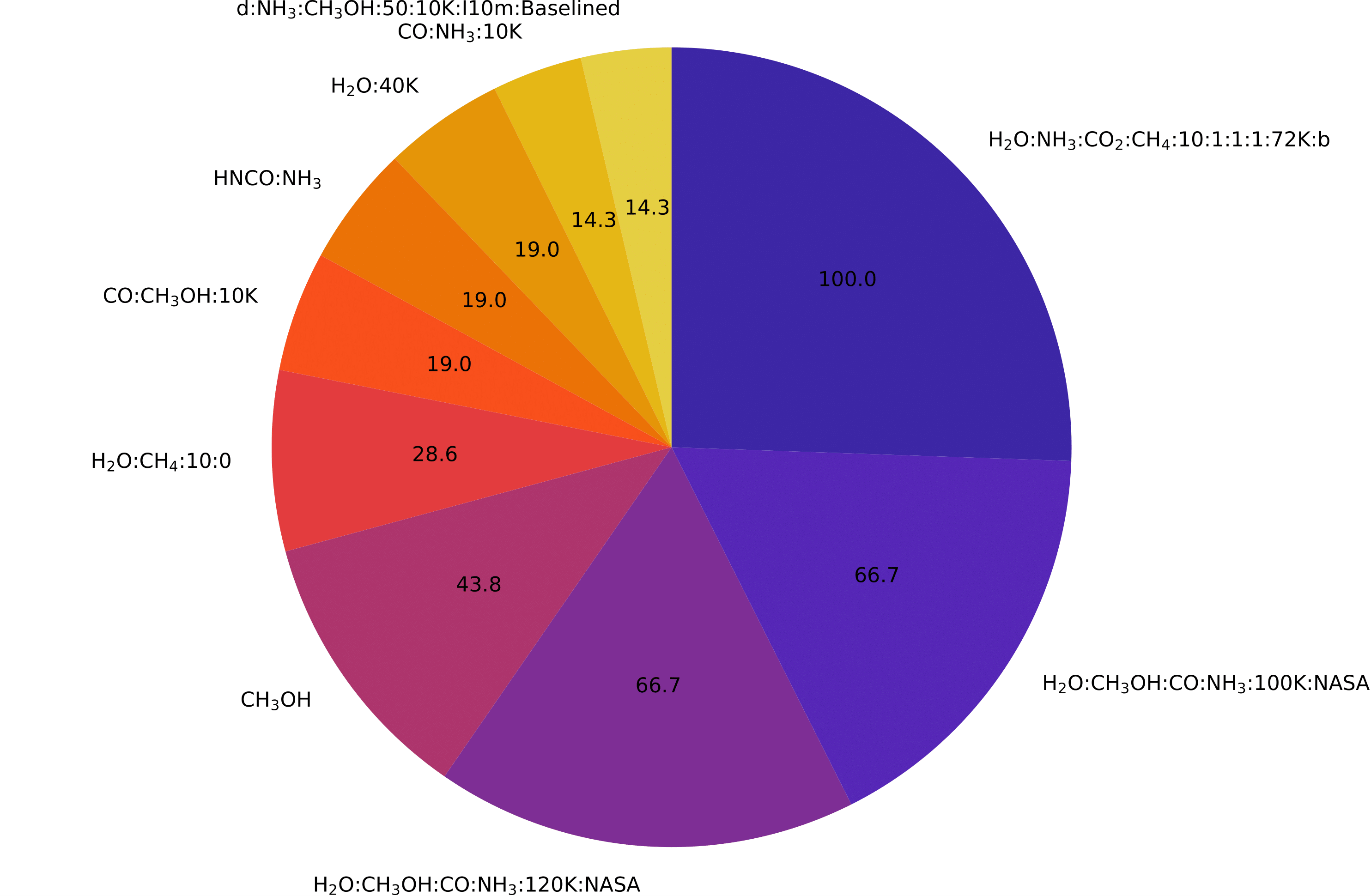
Figure 7: Pie charts of the recurrence plots.

The values are given in percentage and means how many time a specific data was repeated in order to contribute to the selected confidence interval.

Calculating confidence intervals and ice column densities

The confidence intervals can be visualised along with the spectral decomposition plot as follows:

>>> from ENIIGMA.Stats import Stats_Module
>>> Stats_Module.stat(f_sig=2)

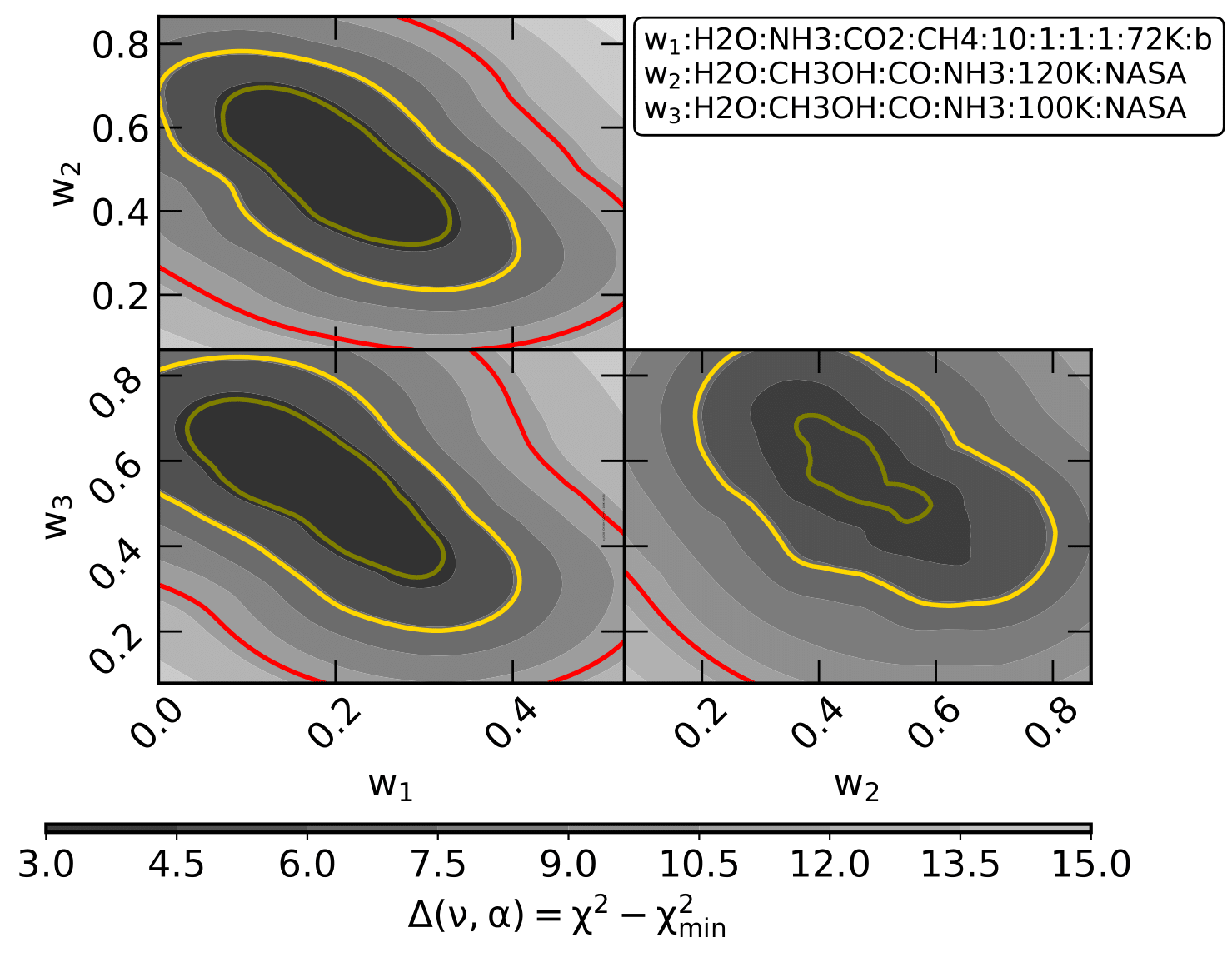
Figure 8: Triangle plot showing the confidence intervals.

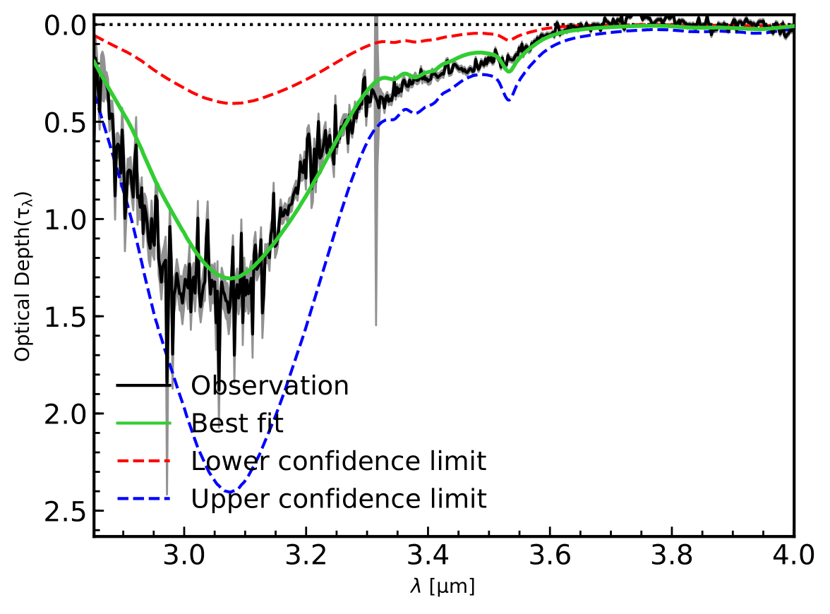
Figure 9: Optical depth and the minimum and maximum intervals.

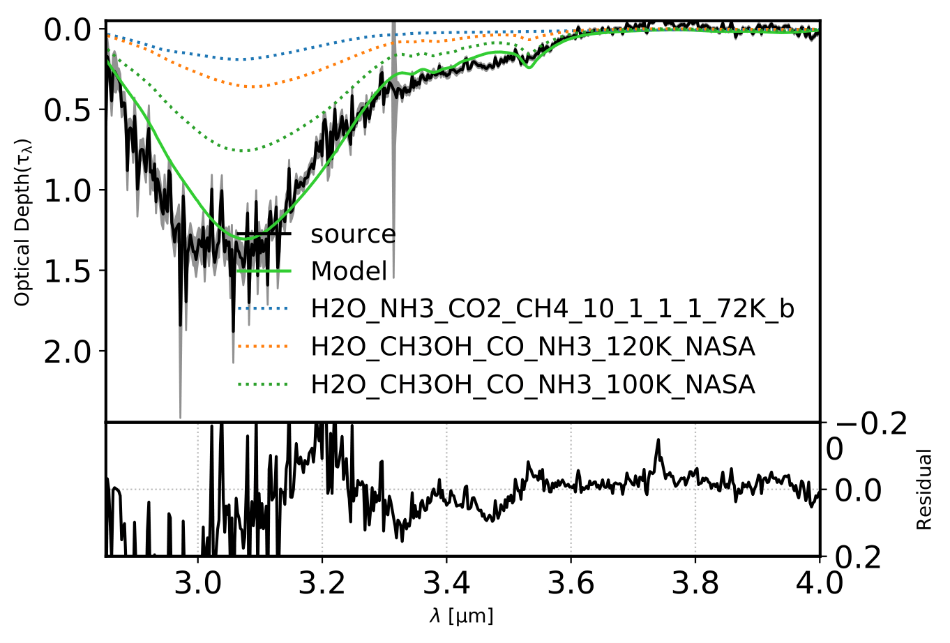
Figure 10: Optical depth decomposition indicating the used experimental data.